I wanted to write a post to make clear in simple and elegant way the singular characteristic of a Topic-Specific PageRank to be composible with respect to the personalization vectors, but I wanted to start from the beginning so I split the entire journey in two posts: the first is this one and we will see the general PageRank motivation and formulation, the second one will deal with the personalized PageRank ones.

What is PageRank

Suppose that you want to rank web pages by assigning them a score that is a degree of their authority and popularity, the fundamental key property of the web graph that you need to consider are links. Links are a measure of popularity, theoretically if you link another web page you consider it authoritative (I’m going link in this article Wikipedia, books, citation resources), moreover it’s rare that a spam page links a good page, in general good pages links good pages and spam pages links other spam pages, this is the links’ nature.

The random walker

But how we can consider links to score pages? It does not suffices to count them since we can easily create spam pages that have lots of in and out links. The brilliant idea of PageRank is to consider the weighted sum of the in-links, but weighted on the base of what? Easy, on the rank of the page from which the link is coming. So in general, for a page \(j\) and for every page \(i\), with out-degree \(d_i\), that points to \(j\) we can express the score of \(j\) as:

Therefore, the amount of rank of the linking page \(i\) is divided equally to all the out links. We can give to this equation a nice interpretation that also allows us to understand why it is not enough. Suppose that we have a random walker, an entity that just walks on our graph with a specific behaviour: regardless on the node on which it stays at a certain time \(t\) it always follows a random link of that node, so the probability that any link of the node will be chosen by the walker is evenly distributed to all the links, did you remember? Even the rank was evenly distributed to all the out links.

We can model the random walker with a Markov chain, a statistical model composed by \(N\) states, where \(N\) is the number of nodes since the walker can be any of them in a certain time \(t\). The key property of a Markov chain is that we can write in an elegant way all the decisions that can be made by the walker at any state by writing down a column stochastic transition probabilities matrix \(M\). Trust me, it seems more difficult than what it actually is.

In the matrix \(M\) every column represents a state in which the random walker can be, in other words, a node, and each row represents the next node in which the walker will be directed, specifically given a column \(j\) and a row \(i\) the cell \(M_{ij}\) is the probability that the next node will be \(i\) given the fact that the walker is on the node \(j\). If you remember, this probability is again evenly distributed to all the out links a node, so you will agree with me that the sum of every column is 1 (that is what column stochastic matrix means). An example will clarify any doubt.

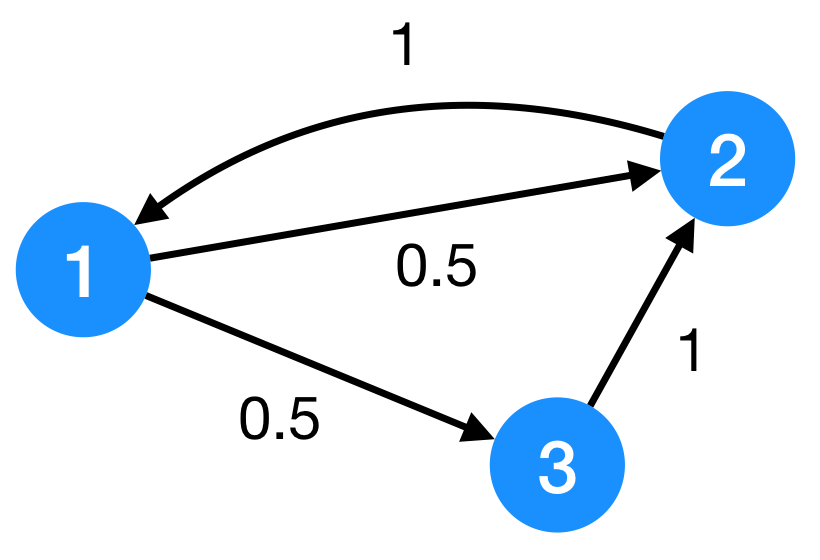
In the graph that is in the figure we can write down the following transition probabilities matrix:

You should notice now that the element of the matrix are just the previous \(\frac{1}{d_j}\) for a row \(j\) and for any link to node \(i\):

Now, given the column vector \(\mathbf{r}\) that contains all the ranks for every page, you will allow me to write the following compact formulation of the PageRank:

And you will see that I also added the concept of time, since we are updating the rank vector \(\mathbf{r}\) at any step of the random walker. Did you see it? Just take your time to see that the matrix formulation is the same of the one that we started with.

The Power Method

How the algorithm would work? We call this method of computing the PageRank the power method since we progressively apply always the same equation on the rank vector \(\mathbf{r}\). We initialize the rank vector as follows:

That is a vector of \(N\) elements in which every element is \(\frac{1}{N}\). You have to think about this vector as the probability of the random walker to be in every node of the graph at certain time \(t\). At the beginning, time 0, the walker can be in any node with a evenly distributed probability (this is why we initialize it in that way), after applying the same equation a lot of times we will have that vector to converge to a steady-state probability vector or also called long-term visit rate, the probability that a node is visited in the long-term, that is another interpretation of the PageRank.

We have:

• Step 0: \(\mathbf{r}^{(1)} = M \cdot \mathbf{r}^{(0)}\)
• Step 1: \(\mathbf{r}^{(2)} = M \cdot \mathbf{r}^{(1)}\)
• Step 2: \(\mathbf{r}^{(3)} = M \cdot \mathbf{r}^{(2)}\)
• ..until convergence

Pathologies

So far so good, we can also prove that the previous formulation converges (see the references at the end of this post if you want to know why). Now everything works with graphs like the one in the example, in general the graph of the web not only is not so simple but also it has two pathological issues:

• It has spider traps, namely there are some structures of nodes that if the walker manages to enter them then it cannot escape because all the pages have links between each other of the same group. This is a problem since the trap will absorbe the PageRank of all the pages, this can also be more pathological if we have cyclic structure since they makes our Markov chain periodic.
• It has dead ends, there are some nodes that have no out links and this is a problem because for a dead end the column for that state is not summing to 1 and the matrix is no more column stochastic. In general if a graph has dead ends then its corresponding Markov chain is reducible meaning that there not exists a path from every node to every other one.

Thus, there are some conditions that must be followed in order to have the convergence to a true PageRank \(\mathbf{r}\): we say that the Markov chain has to be ergodic, namely irreducible and aperiodic.

The cure

The second brilliant idea that fixes all the pathological issues of a web graph was to modify the behaviour of the random walker in such a way when it stays on a node it has two possibilities to be chosen:

• with probability \(\beta\), it follows a random out-link of the node it is on, as in the general formulation;
• with probability \(1-\beta\), it teleports itself to node of the graph chosen at random (so every node is chosen with probability \(\frac{1}{N}\)).

You will realize now that if the walker jumps to random node it can easily escape both from dead ends than spider traps, so the teleporting made our PageRank defined and our iteration method to converge. How our equation will be modified? The equation of a single node \(j\) becomes:

in vector notation we want to modify our matrix \(M\) in order to accomodate the random teleport, therefore we write a new matrix \(A\) that is:

and since \(\mathbf{r}^{(t+1)} = A\cdot\mathbf{r}^{(t)}\) we want to find the final formulation to be applied:

This is the final formulation of the PageRank, notice that in the first step with added a \(N\times N\) matrix \(\left[\frac{(1-\beta)}{N}\right]_{N\times N} \) to simulate the random teleporting, but when we multiply it to the rank vector \(\mathbf{r}\), since it is a stochastic vector (the sum of all coordinates is 1) the previous matrix becomes a vector of \(N\) elements, \(\left[\frac{(1-\beta)}{N}\right]_N\) and the rank vector disappears on the second element of the sum¹.

Practical example

Let’s see this in practice with SageMath code²:

# Number of the nodes
n_nodes = 3
# Transition probabilities matrix
M = matrix([[0,1,0],[0.5,0,1],[0.5,0,0]])
b = 0.9
# Vector of evenly distributed probabilities
p = vector([1/n_nodes for i in range(n_nodes)])

# Init the rank vector with evenly distributed probabilities
r = vector([1/n_nodes for i in range(n_nodes)])

for i in range(1000):
    r = (b*M)*r + (1-b)*p
    
print("r = " + str(r))

This replies with: r = (0.391901663051338, 0.398409255242227, 0.209689081706435)

The dead ends problem

The equation that we have just seen does not work if the graph has dead ends, this because a dead end does not have the the contribution of \(\beta\) probability since it has no out links! For this reason the leaked probability by the dead ends it’s not just \(1-\beta\) but it is larger. So we have two possibilities, or adding the vector \(\frac{1}{N}_N\) to dead ends states of the matrix or splitting the iteration in two steps:

• Step 1: compute the standard PageRank

  \[\mathbf{r}^{(t+1)} = \beta M \cdot \mathbf{r}^{(t)}\]

• Step 2: redistribute the leaked probability evenly by summing all the coordinates of the rank vector and dividing the remaining probability to all the nodes of the graph:

  \[\begin{split} \mathbf{r}^{(t+1)} & = \mathbf{r}^{(t+1)} + (1 - \beta) \cdot \left[\frac{\left(1 - \sum_i r^{(t+1)}\_i\right)}{N}\right]\_N \\\\ & = \mathbf{r}^{(t+1)} + (1 - \beta) \cdot \left(1 - \sum_i r^{(t+1)}\_i\right) \left[\frac{1}{N}\right]\_N \end{split}\]

I prefer to get out the \(\left[\frac{1}{N}\right]_N\) because we will see in the next post that it can personalized as we want for giving a generalization of the PageRank.

Practical example

Again we see an application with SageMath in the following code:

# Number of the nodes
n_nodes = 3
# Transition probabilities matrix
M = matrix([[0,1,0],[0.5,0,1],[0.5,0,0]])
b = 0.9
# Vector of evenly distributed probabilities
p = vector([1/n_nodes for i in range(n_nodes)])

# Init the rank vector with evenly distributed probabilities
r = vector([1/n_nodes for i in range(n_nodes)])

for i in range(1000):
    # Step 1
    r = (b*M)*r
    # Step 2 - distribute the remaining probability
    r = r + (1 - sum(r)) * p
    
print("r = " + str(r))

This replies with: r = (0.391901663051338, 0.398409255242227, 0.209689081706435)

The same result of the previous algorithm.

References

• Mining of Massive Datasets, Jure Leskovec, Anand Rajaraman, Jeff Ullman
• IIR: Introduction to Information Retrieval. Christopher D. Manning, Prabhakar Raghavan and Hinrich Schütze. Cambridge University Press, 2008